Correlation Dynamics and Probabilistic Cellular Automata

Test

Montpellier,October 26, 2001
Cambridge November 11, 2001
Paris May 15, 2002
Edinburgh, June 25. 2002
Paris, February 8, March 8, April 1 2003
Amsterdam, May 28, 2003
Paris, October 23, 2003
Paris, March 19, April 5, April 29, July 3, 2004
Paris, February 8, 2005

This Mathematica notebook gives an overview of what can be done with my cellular automaton and correlation dynamics packages.
More info on the pages on correlation dynamics on my personal website.

•Load Modules

Put the packages in Mathematica's preferred locations or place them together with the notebook. Modify the following so that Mathematica operates in the right directory

In[1]:=

In[2]:=

Out[2]=

In[3]:=

Out[3]=

•Define the Model

We are going to define a model where every site is either empty, occupied by a healthy (sus) or an infected (inf) host:

In[4]:=

Out[4]=

The events that change the states of sites are

In[5]:=

$eventList := {event[ {oc[i_], emp}, {oc[i_], oc[sus]}] :> phi b[i], event[ {oc[i_], x_}, {emp, x_}] :> phi d[i], event[ {oc[sus], oc[inf]}, {oc[inf], oc[inf]}] :> phi beta, event[ {oc[i_], emp}, {emp, oc[i_]}] :> phi m[i]} ;$

which represent reproduction, mortality, infection and movement.

In[6]:=

some definitions for displaying things:

In[7]:=

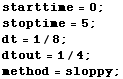
some simulation specifications

In[10]:=

•Run mean field model

In[11]:=

Out[11]=

In[12]:=

Out[12]=

In[13]:=

Out[13]//TableForm=

$-b[inf] p[{emp}] p[{oc[inf]}] + d[inf] p[{emp}] p[{oc[inf]}] + d[inf] p[{oc[inf]}]^2 - b[sus] p[{emp}] p[{oc[sus]}] + d[sus] p[{emp}] p[{oc[sus]}] + d[inf] p[{oc[inf]}] p[{oc[sus]}] + d[sus] p[{oc[inf]}] p[{oc[sus]}] + d[sus] p[{oc[sus]}]^2$

$b[inf] p[{emp}] p[{oc[inf]}] + b[sus] p[{emp}] p[{oc[sus]}] - d[sus] p[{emp}] p[{oc[sus]}] - beta p[{oc[inf]}] p[{oc[sus]}] - d[sus] p[{oc[inf]}] p[{oc[sus]}] - d[sus] p[{oc[sus]}]^2$

$-d[inf] p[{emp}] p[{oc[inf]}] - d[inf] p[{oc[inf]}]^2 + beta p[{oc[inf]}] p[{oc[sus]}] - d[inf] p[{oc[inf]}] p[{oc[sus]}]$

In[14]:=

In[15]:=

In[16]:=

In[17]:=

[Graphics:HTMLFiles/demo.nb_24.gif]

Out[17]=

•Run correlation dynamics version

In[18]:=

Global densities

In[21]:=

[Graphics:HTMLFiles/demo.nb_28.gif]

Out[21]=

Densities as `seen' by the parasite

In[22]:=

[Graphics:HTMLFiles/demo.nb_31.gif]

Out[22]=

•Correlation dynamics equations

In[23]:=

Out[23]=

In[24]:=

Out[24]=

In[25]:=

Out[25]=

In[26]:=

Out[26]=

In[27]:=

Out[27]=

These equations can be worked a bit more to look like proper correlation dynamics equations, but Mathematica remains rather limited in its capacity to represent symbolic output.

•Run explicit PCA simulations

Define temporal...

In[28]:=

... and spatial aspects of the simulation

In[33]:=

where to store the results

In[36]:=

... and put together parameter files instructing the external module simpca

In[37]:=

In[38]:=

Out[38]=

(This takes a long time, but using Mathematica for this kind of simulation is like using a gun to kill a mosquito, whatever its original author might say)

Global and local densities:

In[39]:=

[Graphics:HTMLFiles/demo.nb_74.gif]

Out[39]=

In[40]:=

[Graphics:HTMLFiles/demo.nb_77.gif]

Out[40]=

•Run external PCA simulations

In[41]:=

Where to store the results

In[42]:=

... and put together parameter files instructing the external module simpca

In[43]:=

In[44]:=

In[45]:=

The following two commands read from file the simulation results

In[46]:=

In[47]:=

Global and local densities

In[48]:=

[Graphics:HTMLFiles/demo.nb_93.gif]

Out[48]=

In[49]:=

[Graphics:HTMLFiles/demo.nb_96.gif]

Out[49]=

•Compare the results

with mean field model

In[50]:=

[Graphics:HTMLFiles/demo.nb_99.gif]

Out[50]=

with correlation dynamics model

In[51]:=

[Graphics:HTMLFiles/demo.nb_102.gif]

Out[51]=

Now, compare predictions about the local environment of parasites

In[52]:=

[Graphics:HTMLFiles/demo.nb_105.gif]

Out[52]=

•Make snapshot of lattice

In[53]:=

$plotState[emp, pos_] := {GrayLevel[1], Disk[pos, 0.4]} plotState[oc[x_], pos_] := {color[x], Disk[pos, 0.4]}$

In[55]:=

Out[55]=

In[56]:=

[Graphics:HTMLFiles/demo.nb_111.gif]

Out[56]=

In[57]:=

•An Allee effect

To show how vital rates can be density dependent, let us introduce an Allee effect

In[58]:=

$eventList := {event[ {oc[i_], emp}, {oc[i_], oc[sus]}] :> phi b[i] (phi 2 (1 - nb[emp, $focus]))^2, event[ {oc[i_], x_}, {emp, x_}] :> phi d[i], event[ {oc[sus], oc[inf]}, {oc[inf], oc[inf]}] :> phi beta, event[ {oc[i_], emp}, {emp, oc[i_]}] :> phi m[i]} ;$

here it is assumed that birth rates increase with double the square of local density (phi is one over the number of neighbours)

In[59]:=